25 Feb Pearson and Spearman Correlations in R
In a previous post we explained the concept of correlation between two variables and specifically discussed for Spearman and Pearson correlations. Here, we will have a practical example using R language.
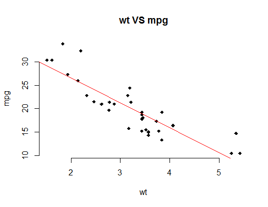
With the following script we create a scatter-plot derived from two columns of the mtcars dataset depicting the relationship of weight(wt) and miles per gallon(mpg).
> x <- mtcars$wt
> y <- mtcars$mpg

#scatter plot
> plot(x, y, main = "wt VS mpg",
     xlab = "wt", ylab = "mpg",
     pch = 18, frame = FALSE)
> abline(lm(y ~ x, data = mtcars), col = "red")

Assumptions
Pearson correlation is a parametric correlation and can be used only when x, y come from a normal distribution. In our example, we can test this assumption using the Shapiro-Wilk normality test.
# Shapiro-Wilk normality test for wt
> shapiro.test(x)

	Shapiro-Wilk normality test

data:  x
W = 0.94326, p-value = 0.09265

# Shapiro-Wilk normality test for mpg
> shapiro.test(y)

	Shapiro-Wilk normality test

data:  y
W = 0.94756, p-value = 0.1229
In this test, the null hypothesis is that the data come from a normal distribution. In case when p-value < 0.05 we can reject the null hypothesis and accept the alternative one. Here, for both x and y we accept the null hypothesis and x,y are normally distributed.
Correlations
Calculating the Pearson and Spearman correlations with the following lines, we have:
#pearson
> cor(x,y,method = "pearson")
[1] -0.8676594

#spearman
> cor(x,y,method = "spearman")
[1] -0.886422
Both of these metrics indicate strong correlation between weight and mpg variables of the mtcars dataset. Spearman has a slightly higher value since it captures the monotonic relationship and not strictly the linear relationship.


Sorry, the comment form is closed at this time.