Linear Regression Modeling with R

Last time we made a gentle introduction to linear regression model theory and also discussed about the assumptions that must hold true for a well defined linear model. In this post, we will use an actual dataset and will fit a linear model to it and explain our findings.

We will use the cars dataset which is imported in R by default. It is a simple datset with two columns; speed and distance. Below we can see the five first rows of the datset;

>head(cars)
speed dist
1 4 2
2 4 10
3 7 4
4 7 22
5 8 16
6 9 10

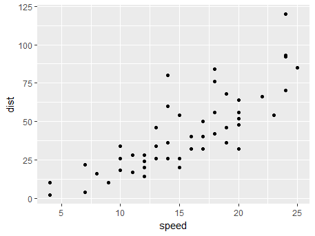
Now we will visualise the dataset in a scatter plot to see if there is a linear relationship;

ggplot(cars, aes(x=speed, y=dist)) + geom_point()

We can see that there is a clear linear relationship between speed and distance variable in the cars dataset, something that is verified by the value of linear correlation of 0.8068.

Modeling

Now that we know that there is a linear relationship in the dataset, we will build a linear model with the following line of code:

>linear_mod <- lm(dist ~ speed, data=cars) # build linear regression model 
>print(linear_mod)

Call:
lm(formula = dist ~ speed, data = cars)

Coefficients:
(Intercept)        speed  
    -17.579        3.932  

Inspecting the output of the model, we can see that:

dist = −17.579 + 3.932∗speed

Diagnostics

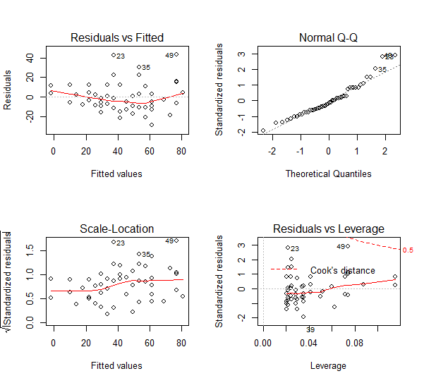
With the next command we are plotting some standard diagnostic plots to check if the assumptions of the linear model are met;

> par(mfrow = c(2, 2))
> plot(linear_mod)

From the upper right plot (Q-Q plot) we can see that the normality assumption is met for the residuals since they are normally distributed. Also, from the upper left plot, we would expect that the residuals will have constant variance when plotted against fitted values and absence of any pattern (funnel) or trend. In our example, the residuals seem to have a small but negligible variance. On the lower right plot we have the leverage vs residuals plot. Leverage is a metric revealing the amount of influence of a particular value to the resulted model. Points in the plot with high leverage and absolute residual values are considered as outliers. In our example all the points are within the Cook’s distance line (dashed red line) and therefore are not that influeantial to the model. Lastly, the lower left plot is another version of the residuals vs fitted plot and should be no trends in this. Indeed, in our plot, no discrenible trends exist.