14 Jan A Brief Introduction to Linear Regression
In this post we will discuss about one of the most important and widely used econometrics models, the linea regression. Through a series of posts, we start by the definition and then we will explain further the mathematical notation and equations describing the model. Of course we will showcase examples using R and discuss on model diagnostics in future posts.
Definition
Linear regression attempts to model a relationship between a response (dependent) variable and a single (or multiple) predictor (independent) variables. In the case of multiple predictors, the process is called multiple linear regression. Generally, linear regression is used in two main scenarios: a) to determine if a set of predictors does a good job in predicting a response variable b) to explicitly detect those predictors with the greatest predictive ability over the response variable.
Mathematical derivation
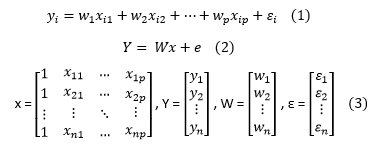
Assuming we have the following dataset: {yi,xi1,…,xip} where i is the number of the examples available and p is the number of predictors, then the equation describing the relationship of y with multiple predictors x is shown in equation (1) in the following image. Equation (2) shows equation (1) in matrix notation and equations (3) highlight the matrices used in equation (2).

Ordinary least squares
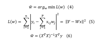
Ordinary least squares is method for estimating the unknown variables in a linear regression process (in our case the variable w). It is based on the principle of minimizing the squared errors of the differences between the actual and predicted values (equation (4)). The problem is a quadratic optimization process which is convex and always has a solution. The mathematical notation is as given by equation (5) in scalar and matrix form and and the optimal solution is given by matrix by equation (6) in matrix form.


Sorry, the comment form is closed at this time.