03 Feb Beyond Linear Modeling using R (part-1)
Many problems in econometrics are based on the assumption that two (or more) observed variables have linear dependency with each other. However, this is not applicable in every case. Non-linear relations are equally probable. In this series of posts, we will highlight some cases and ways to fit non-linear models using R.
First, we will generate some data for two variables x and y:
# generate data
> set.seed(1)
> length <- 30
> x <- runif(length)
> y <- x^3 + rnorm(length, 0, 0.06)
> ds <- data.frame(x = x, y = y)
> str(ds)

'data.frame':	30 obs. of  2 variables:
 $ x: num  0.266 0.372 0.573 0.908 0.202 ...
 $ y: num  0.016 0.0506 0.2446 0.7984 0.0438 ...
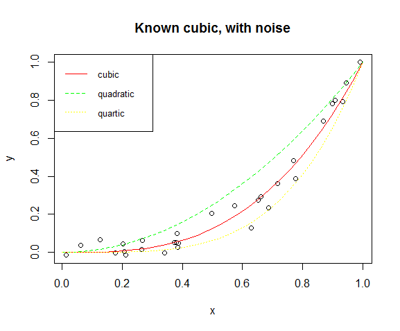
Now we will visualise the dataset in a scatter plot to see the non-linear relationship and also we will draw quadratic, cubic and quartic lines with red, green and yellow colors respectively:
# plotting
> plot(y ~ x, main = "Known cubic, with noise")
# Add lines
> lines(s, y1, col="red", lty=1)
> lines(s, y2, col="green", lty=2)
> lines(s, y3, col="yellow", , lty=3)
# Add a legend
> legend("topleft", legend=c("cubic", "quadratic", "quartic"),
       col=c("red", "green", "yellow"), lty=1:3, cex=0.8, box.lty=1, box.lwd=1)

Modeling
Clearly, the relationship between x, y is exponential and can be described by the following mathematical form:
In order to built a model that will appropriately describe the above mathematical formula, we will use the function nls() as follows:
# non-linear modeling
> nlmodel <- nls(y ~ I(x^power), data = ds, start = list(power = 1),trace = F)
# summary
> summary(nlmodel)

Formula: y ~ I(x^power)

Parameters:
      Estimate Std. Error t value Pr(>|t|)
power   3.0470     0.1188   25.65   <2e-16 ***
---
Signif. codes:  0 ‘***’ 0.001 ‘**’ 0.01 ‘*’ 0.05 ‘.’ 0.1 ‘ ’ 1

Residual standard error: 0.04676 on 29 degrees of freedom

Number of iterations to convergence: 5
Achieved convergence tolerance: 4.257e-07
Inspecting the output of the summary() result, we can see that the value of the power is 3.047 ± 0.1188 and is highly significant. The magnitude of the standard error is a measure of uncertainty for the estimated value of the exponent.
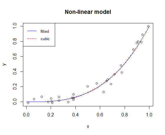
Fitting the model obtained above and stored in nlmodel and plotting the lines we have the following graph:
plot(y ~ x, main = "Non-linear model")
lines(s, s^3, lty = 2, col = "red")
lines(s, predict(nlmodel, list(x = s)), lty = 1, col = "blue")
legend("topleft", legend=c("fitted", "cubic"),
       col=c("blue", "red"), lty=1:2, cex=0.8, box.lty=1, box.lwd=1)

We can see that the fitted model is very close to the cubic model that we used to create the data with the additional noise.
Goodness of fit
To examine the goodness of fit of the model, we will calculate R squared, seen in a previous post for linear regression:
# sum of squared error
> SSE <- sum(residuals(nlmodel)^2)
# total sum of squares
> SST <- sum((y - mean(y))^2)
# Rsquared
> Rsquared <- 1-(SSE/SST)
R squared is calculated at 0.9778 which is a very good result highlighting the overall good performance of the model.


Sorry, the comment form is closed at this time.